VLOOKUP Date Range and Return Value in Excel (4 Suitable Methods) (2024)

Often you may need to VLOOKUP dealing with the date. If you want to return a certain value or values for the date range instead of VLOOKUP by date, you’re here in the right place. In this article, I’ll show 4 methods to VLOOKUP date range and return value in Excel with the necessary explanation. So that you can adjust the methods for your uses.

Download Practice Workbook

4 Methods to VLOOKUP Date Range and Return Value in Excel

Let’s introduce today’s dataset where the name of the Items is provided along with Order Dates, Unit Price, Quantity and Sales. Here, I used some future dates which don’t hamper the analysis.

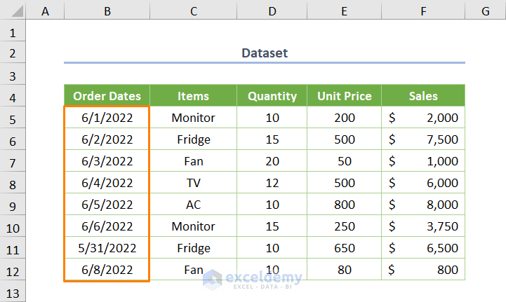
Now, you’ll see the methods on how to VLOOKUP based on the date range (i.e. Order Dates) and then return the corresponding value. Right before that, I’d like to say that I’ll show you 2 methods using the VLOOKUP function (1st and 3rd methods). Besides, you’ll see the use of INDEX and MATCH functions in the second method. Lastly, the application of the LOOKUP function will be discussed.

Let’s dive into the methods.

1. VLOOKUP a Date within Date Range and Return Value

In the first method, you’ll explore the way of finding value if you specify a date within the date range. Let’s say, your lookup date within the date range (i.e. Order Dates) is in the D14 cell. Then, you want to return the value of the Sales of the corresponding cell (Lookup Order Date).

Truthfully, it’s a simple method. Just use the following formula in the D15 cell.

Here, D14 is the lookup order date, B5:F12 is the table array, 5 is the column index number (you may visit VLOOKUP Column Index Number if you have any confusion with this argument), and finally TRUE is for approximate matching.

Read More: How to Use Formula for Past Due Date in Excel (3 Methods)

2. Find a Single Output Dealing with Two Dates

Besides, if you want to find a single value covering two dates within the date range in excel, this method will be handy for you. For example, you have to find the output (Sales) having the Order Date greater than 6/3/2022 but less than 6/5/22.

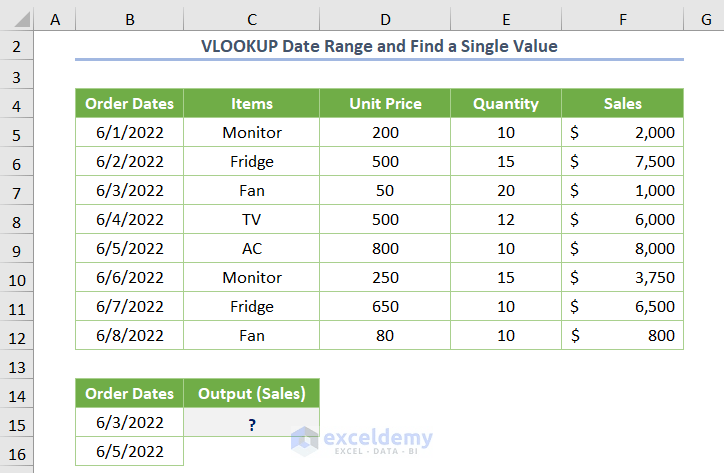
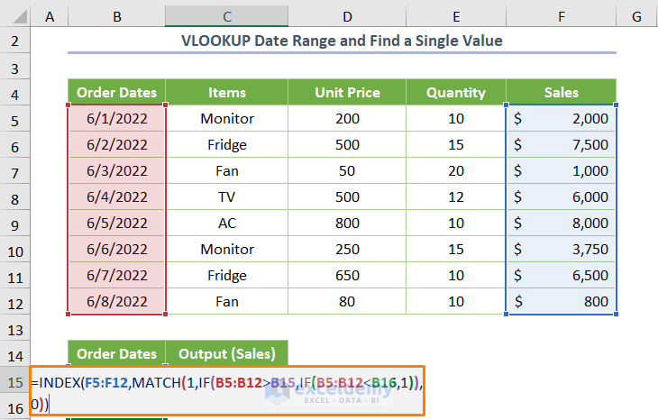
For finding the output, insert the following formula exactly in the C15 cell.

Here, F5:F12 is the cell range for the Sales data, B5:B12 is the cell range for Order Dates, B15 is a date within the date range and B16 is another date within the date range.

In the above formula, the IF logical function returns 1 if the cell fulfills the criteria (greater than but less than). Next, the MATCH function provides the location of the matched values. Finally, the INDEX returns the value of the Sales that fulfills all criteria.

After inserting the formula, if you press ENTER, you’ll get the following output.

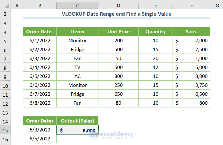
Note: If you want to use this method for a specific date within the date range, you can find that also. In that case, you have to insert the same date instead of the second date.

Read More: VBA to Pivot Table Filter Between Two Dates in Excel

3. VLOOKUP Date Range with Multiple Criteria and Return Multiple Values

More importantly, if you want to return multiple values rather than returning a single value that fulfills multiple criteria in the case of the date range, this method will provide you with outstanding performance.

Assuming that you want to apply the VLOOKUP function to return all values that fulfill the specific date range. As the process of executing the task is a little bit large, just follow the step-by-step guideline.

Step 01: Specifying the Start and End Dates

Initially, you have to specify the Start Date and End Date. In such a situation, using the Name Manager might be useful for updating the data frequently.

➤ Firstly, just type two dates in two different cells as shown in the following picture.

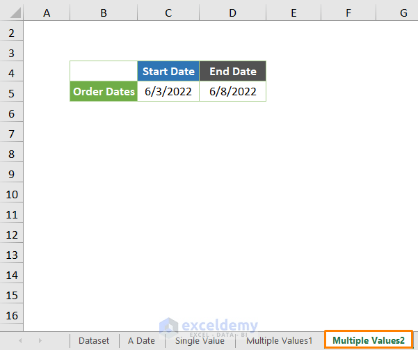
Note: I opened a new working sheet for doing the task. However, it is not mandatory. You can accomplish the same task within the existing working sheet.

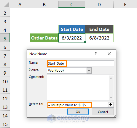
➤ Secondly, select the C5 cell which shows the Start Date, and choose the Name Manager from the Formulas tab.

Immediately, you’ll see a dialog box namely Name Manager and click on the New option.

Next, input the name as Start_Date, and repeat the same process for the End Date.

Step 02: Dealing with the Multiple Criteria of the Date Range

As you know we have to consider dates that fulfill the criteria. The criteria are that the Order Dates would be greater than or equal to Start Date and less than or equal to End Date.

➤ To deal with such criteria, just utilize the IF function.

Here, AND function returns dates that fulfill two criteria. Furthermore, if the criteria are fulfilled, the IF function returns Yes. Else, it will return No.

Step 03: Counting the Lookup Value

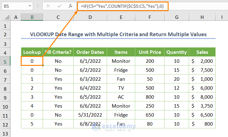
➤ The following combined formula utilizes the IF and COUNTIF functions to count the lookup value if the cell fulfills criteria (matches Yes). Else, it will return 0.

Here, C5 is the starting cell of the Lookup field.

Step 04: Returning Multiple Values

Initially, copy the name of all fields (not the values) in the previous step except the Fill Criteria.

Then enter the lookup value sequentially in the Lookup# field.

Next, go to the C15 cell and insert the following formula.

Here, $B15 is the value of the Lookup# field, $B$4:$H$12 is the table array, C$14 is the lookup value, $B$4:$H$4 is the lookup array, 0 is for the exact matching.

In the above formula, the MATCH function finds the column index number actually for the VLOOKUP function. Finally, the VLOOKUP function returns a matched value of the Order Dates.

Note: You have to specify the dollar sign ($) carefully, otherwise you’ll not get your desired output.

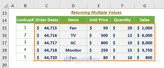
➤ After pressing ENTER, you’ll get the output is 44715. Then, drag the plus sign to the adjacent columns until the Sales and the below cells until the lookup value is 5 (use the Fill Handle Tool).

➤ After dragging down and right, you’ll get the following output.

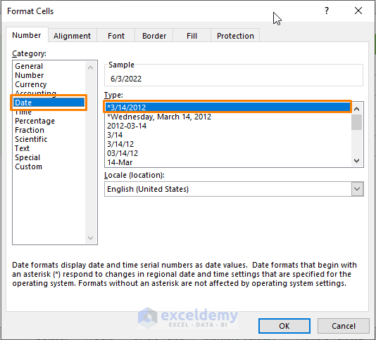
➤ If you look closely, you’ll find that Order Dates are in number format. Just press CTRL + 1 after selecting the cell range C15:C19 to open the Format Cells option.

➤ Then, choose your desired format.

➤ Finally, you’ll get all the values that fulfill the criteria of the date range.

Read More: How to Use IF Formula for Date Range in Excel (6 Methods)

Similar Articles

• How to Use SUMIFS to SUM Values in Date Range in Excel
• Calculate Date Range in Excel
• How to Do SUMIF Date Range Month in Excel (9 Ways)

4. VLOOKUP Two Date Ranges Using the LOOKUP Function

Last but not the least, you also may deal with two different date ranges. For example, I have added an individual column namely Delivery Date. Now, I want to find the specific item that meets two certain dates of the two date ranges. Luckily, you can accomplish the task using the LOOKUP function easily.

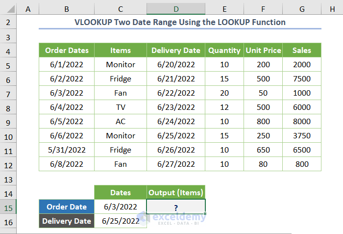
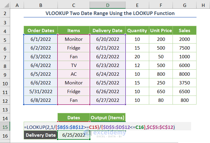
Just insert the following formula.

Here, $B$5:$B$12 is the cell range of the Order Dates, $D$5:$D$12 is the cell range for the Delivery Dates, C15 is an order date and C16 is delivery date. Finally, $C$5:$C$12 is the cell range for the Items.

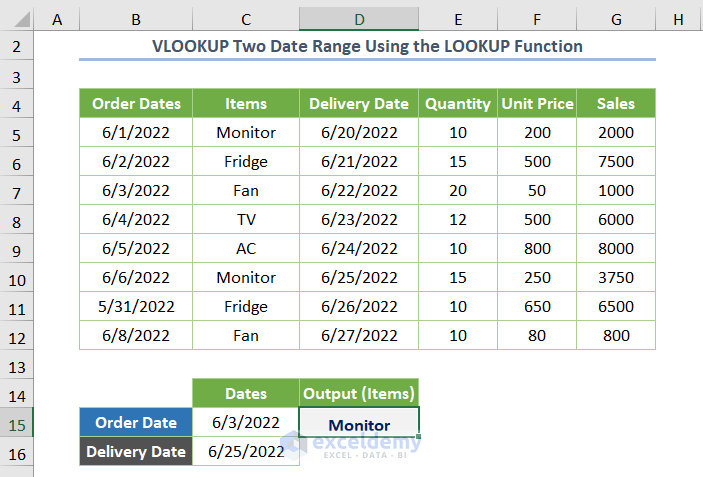
After inserting the formula, you’ll get the following output.

Read More: How to SUMIF between Two Dates and with Another Criteria (7 Ways)

Conclusion

This is how you may apply the VLOOKUP to return a value for the date range in Excel. I strongly believe this article will articulate your Excel journey. Anyway, if you have any queries or recommendations, please share them in the comments section.

Related Articles

• How to Filter Date Range in Pivot Table with Excel VBA
• Set Due Date Reminder in Excel (3 Quick Methods)
• How to Use Pivot Table to Filter Date Range in Excel (5 Ways)
• Calculate Average If within Date Range in Excel (3 Ways)
• Excel VBA: Filter Date before Today (With Quick Steps)